Introduction
Last semester I took a course in Parallel Programming with Dr. Kotsireas and for our final project we wrote a Python program to create high resolution (10,000 x 10,000 pixels) images of Julia sets. We made some pretty pictures and even created a few 3D printed models. After spending the last month updating our code we presented some results in the form of a poster and a few 3D models at the diTHINK 2016 conference in Toronto.
Julia sets are named after Gaston Julia; a French mathematician who helped create the foundations of iteration and fractal theory. Julia sets are created by computing the orbit of a specific value (apply a function to the value, apply the function to the result, etc). Values whose iterations don’t converge are part of the Julia set. Those that do converge are part of the Fatou set.
The functions that are most often used are polynomials of the form $$z^n+c$$ or trig functions like $$c\times\sin{z}$$ where c is a constant st $c\in Complex$ and $n\in Reals$
Math can be used to show that for polynomial functions if the function spits out an absolute value $>=2$ then the subsequent crankings will go to infinity. For sin and cos the same holds if the absolute value of the imaginary part is $>= 50$.
The simplest visualization of Julia Set is to color all values that are part of it black and every else white. If you want to make interesting pictures you can color pixels according to how many iterations it took before the orbit crossed the above mentioned thresholds.
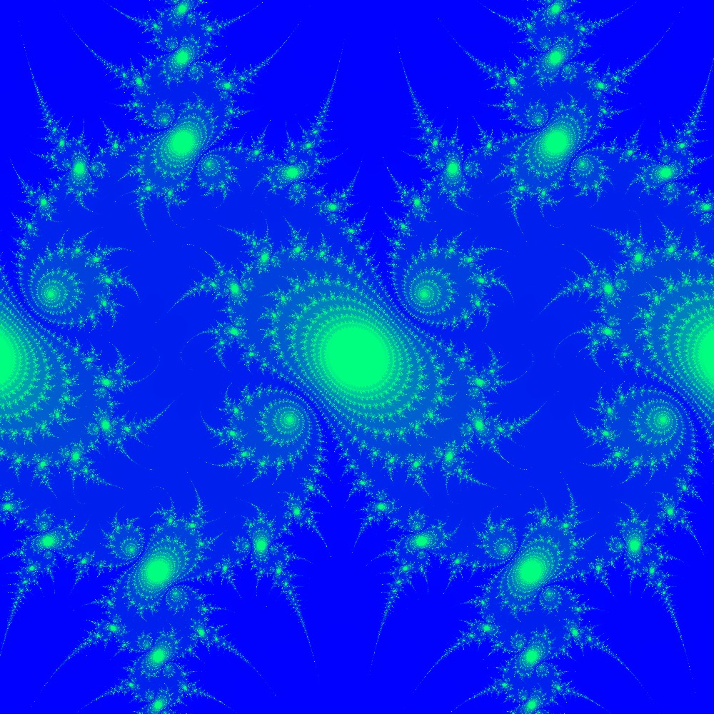
For example

Visualization of the Julia set for the function $z^2 + (-1 + 0i)$
if we turn it into a 3D model we get something like
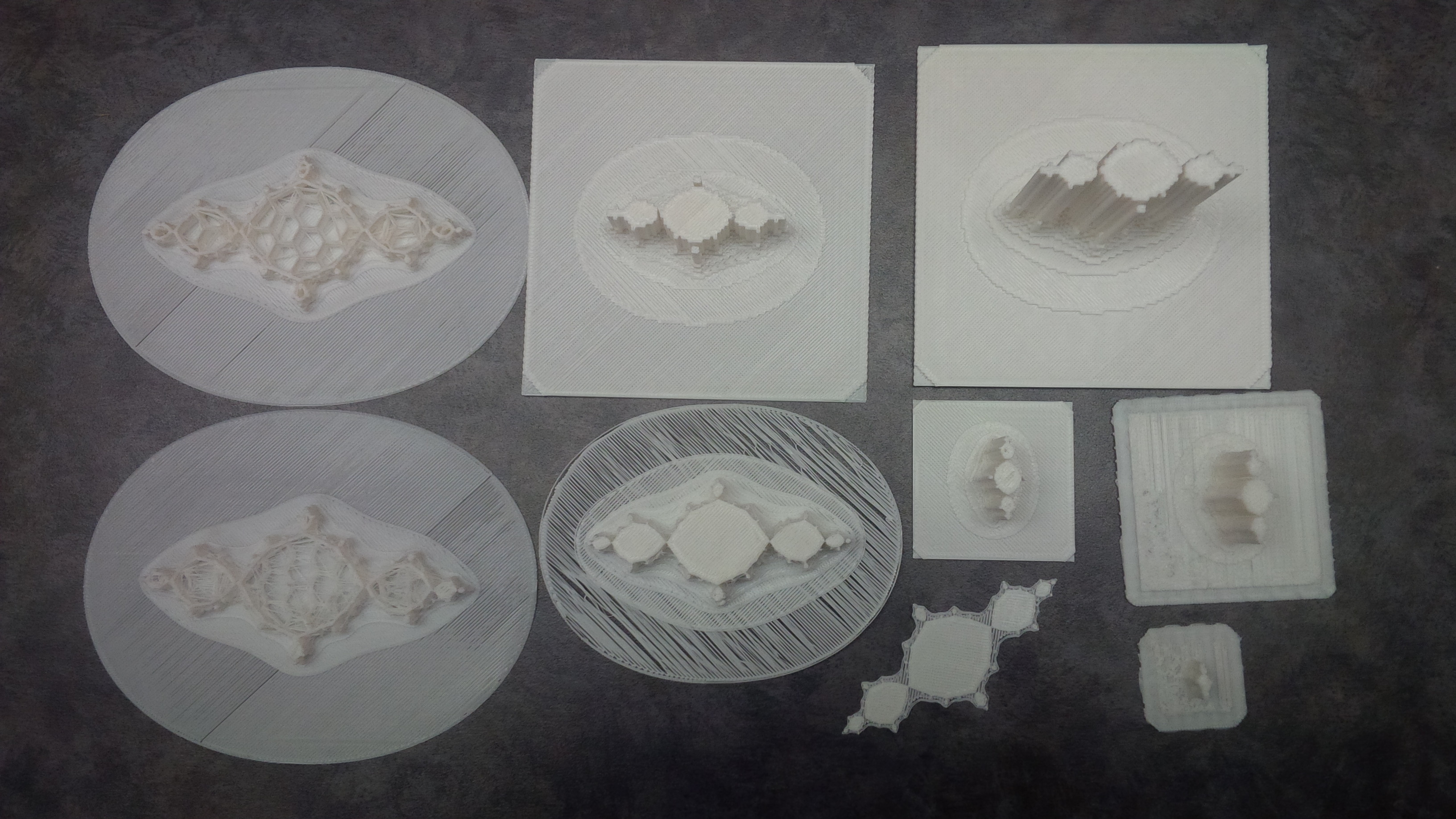
3D Models of $z^2 + (-1 + 0i)$
Raw Data Computation
Naive Simple Method
The simplest way to create the raw data for a Julia set is to use two loops and loop through every initial $x + y\cdot i$ pair. We then use a third loop to compute the orbit of this value and stop when we cross the threshold to infinity or reach our maximum number of iterations.
for x_index, x in enumerate(x_vals):
    for y_index, y in enumerate(y_vals):
        z = complex(x,y)
        iterations = 0
        while abs(z) < threshold and iterations < max_iterations:
            z = z**n + c
            #or z = c*sin(z) or z = c*cos(z)
            iterations += 1
        data[y_index, x_index] = iterations
Note that n is a real number and if using sin or cos use the numpy versions not the built in math versions
Data can be defined as a numpy array using
import numpy as np
data = np.zeros( (num_y, num_x), dtype=np.uint8 )
Note that the data type for the iterations matrix can be set to something else if you want more iterations
Clever Matrix Method
We can make the code more complex and using numpy’s ability to apply functions to entire matricies at once.
x_values, y_values = np.meshgrid( xvals, yvals )
vals = np.zeros( (num_y, num_x), dtype=np.complex )
vals = x_values + y_values*1j

iterations = np.zeros( (num_y, num_x), dtype=np.uint8 )
for i in range(max_iterations):
    vals = vals**n + c
    np.place( vals, abs(vals)>=cutoff, np.nan )
    iterations += np.logical_not( np.isnan(vals) )
The tradeoff is that we need more raw memory to store the intermediate matricies. And it turns out that the code is only faster (as currently written and unoptimized) for small max iteration values.
Approximation Method
We can also theoretically approximate a Julia set by computing one iteration of each orbit and then rounding the resulting values to the nearest grid point. We can then create a graph and figure out the distance between any given point and the infinity node.
Image Creation
The actual images can be created using the Python Image Library.
from PIL import Image
import numpy as np

final_image = np.zeros( (num_y,num_x), np.uint32)
#do something to final image
#...
#export
pilImage = Image.frombuffer('RGBA', final_image.shape, final_image,'raw','RGBA',0,1)
pilImage.save( out_file )
Here it makes sense to use Numpy’s matrix methods to compute the final image.
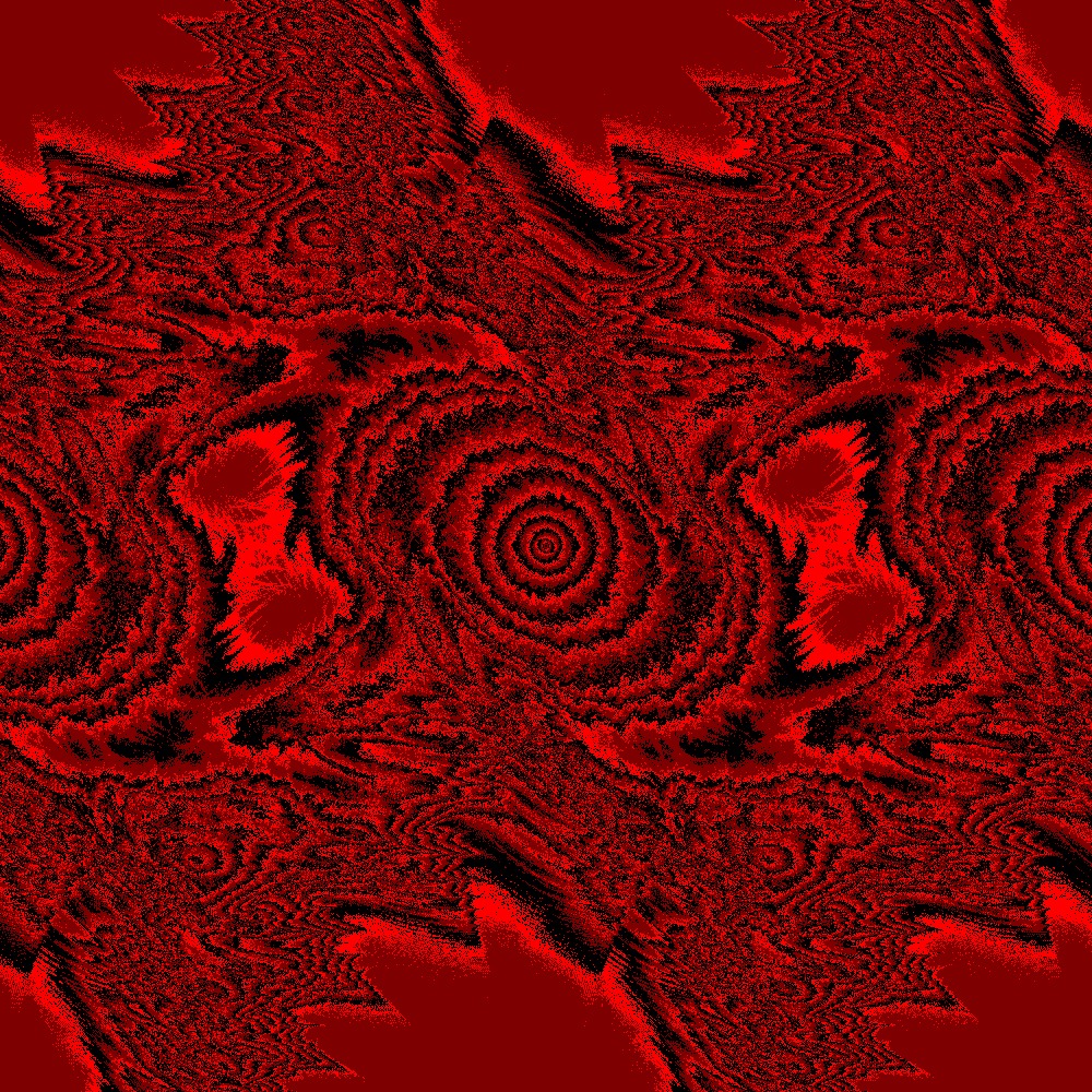
For example to color the image using only red (0 iterations = black, max iterations = brightest red)
final_image += ( (0xFF*iterations.astype(float)/max_i).astype(int)+0xFF000000).astype('int32')
Remember to add your pixel value to 0xFF000000 if you want it to be visible.
If we want to use a built in color map from matplotlib we can do
colors = color_map(iterations.astype(int) )#get colors
colors = colors.reshape( (colors.shape[0]*colors.shape[1],colors.shape[2]) )
colors = (0xFF*colors).astype(int)#Convert to int values for red,green,blue,alpha
final_image += ( sum( colors[:,i]<<(8*i) for i in range(4) ) ).reshape(image.shape)#reverse order and add
3D Models
3D models can be created by creating voxels (3D pixels) for each of the raw data values. Our code places a face on the top of each voxel at the height given by the raw data and adds edge faces whose bottom edge lines up with the next neighbour over. Final edges are dropped to zero. Unfortunately our code is really inefficient for chunks of raw data that are all the same resulting in massive files which take forever to slice. The code also somehow generates holes and other defects which when combined with the inefficient model definition make anything much larger then 100x100 pixels unprintable. That said I’m quite pleased with our STL writer code. I created it as a blend from two different pieces of code.
writer = STL_Writer( out_file )

x_edge = (num_x//2)*x_scale + x_scale/2
y_edge = (num_y//2)*y_scale + y_scale/2

x_grid = np.linspace(-x_edge, x_edge, num_x+1)
y_grid = np.linspace(y_edge, -y_edge, num_y+1)

left_x  = np.column_stack( (x_grid[0:-1],)*num_x ).transpose()
right_x = np.column_stack( (x_grid[1:],  )*num_x ).transpose()

top_y   =  np.column_stack( (y_grid[:-1],)*num_y )
bot_y   =  np.column_stack( (y_grid[1:],  )*num_y )

#top faces points #All have norm (0,0,1)
p4 = np.dstack( (left_x,  bot_y, data) )
p3 = np.dstack( (left_x,  top_y, data) )
p2 = np.dstack( (right_x, top_y, data) )
p1 = np.dstack( (right_x, bot_y, data) )

norm = np.array( [0,0,1]*(p1.shape[0]*p1.shape[1]) ).reshape( p1.shape )
#Top face triangles (defined counter clockwise)
triangles_1 = np.dstack( (norm, p1,p2,p3) )
triangles_2 = np.dstack( (norm, p1,p3,p4) )
triangles = np.vstack( (triangles_1, triangles_2) )

#Export top triangles
triangles = triangles.reshape( ( triangles.shape[0]*triangles.shape[1],12) )
writer.add_faces(triangles)
The only difference for the edges is that they need the neighbour points and the inner points are treated differently then the edge ones.
#-------------------------------------------------------------
#front face points (Not including bottom row)
#-------------------------------------------------------------
p4 = np.dstack( ( left_x[:-1,:],  bot_y[:-1,:],  data[1:,:]) )#use next row down for h
p3 = np.dstack( ( left_x[:-1,:],  bot_y[:-1,:],  data[:-1,:]) )
p2 = np.dstack( (right_x[:-1,:],  bot_y[:-1,:],  data[:-1,:]) )
p1 = np.dstack( (right_x[:-1,:],  bot_y[:-1,:],  data[1:,:]) )
...
#-------------------------------------------------------------
#front face points (Botttom row)
#-------------------------------------------------------------
p4 = np.dstack( (left_x[-1,:], bot_y[-1,:], np.zeros( (1,num_x) )) )
p3 = np.dstack( (left_x[-1,:], bot_y[-1,:], data[-1,:]) )
p2 = np.dstack( (right_x[-1,:], bot_y[-1,:], data[-1,:]) )
p1 = np.dstack( (right_x[-1,:], bot_y[-1,:], np.zeros( (1,num_x) )) )
...
The same idea goes for the other edge faces
Some more pretty pictures
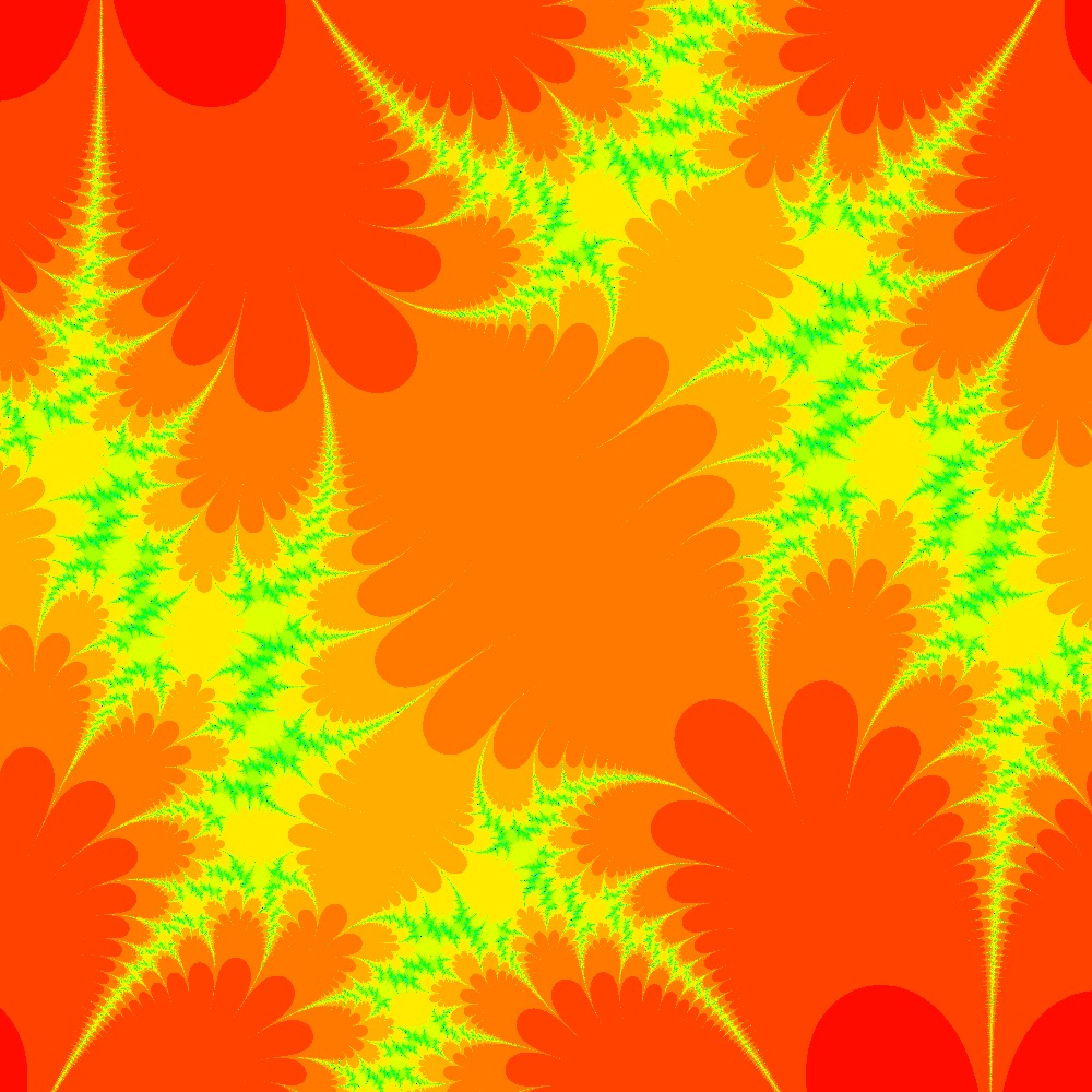
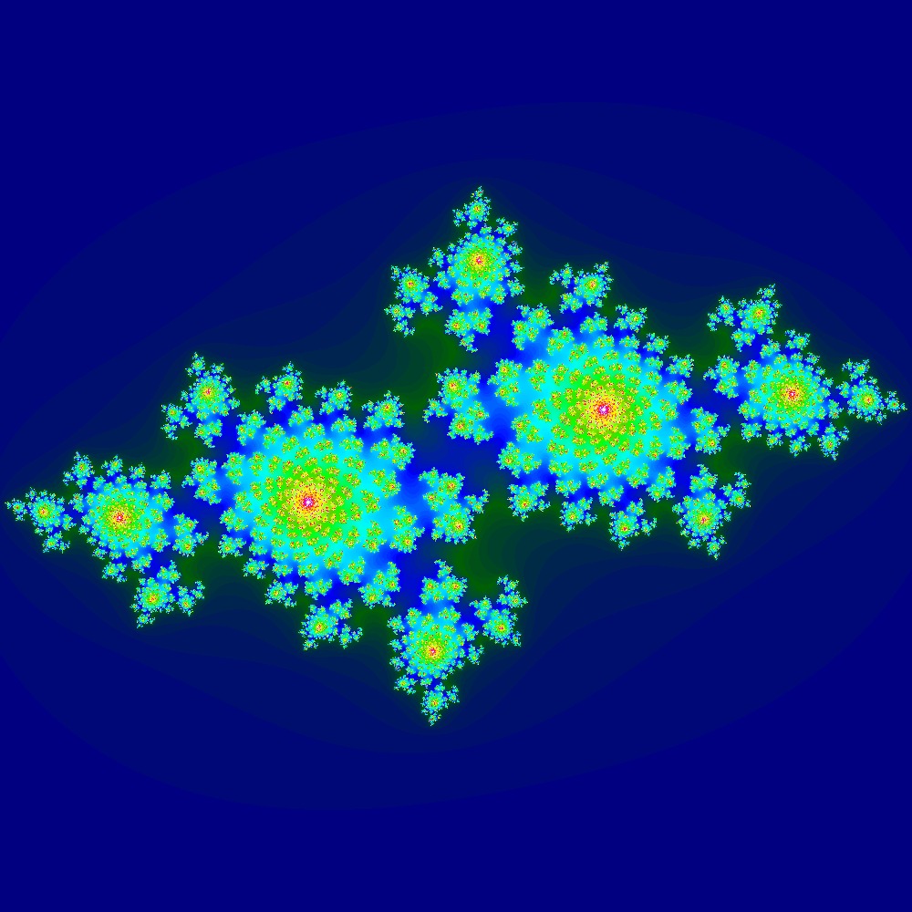
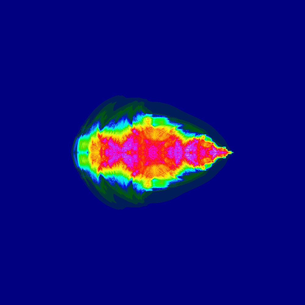
Visualization of the Julia set for the function $c\times sin(z)$ $c=(1+0.1j)$
Visualization of the Julia set for the function $c\times sin(z)$ $c=(1+[0.0..1.0]j)$ 100slices
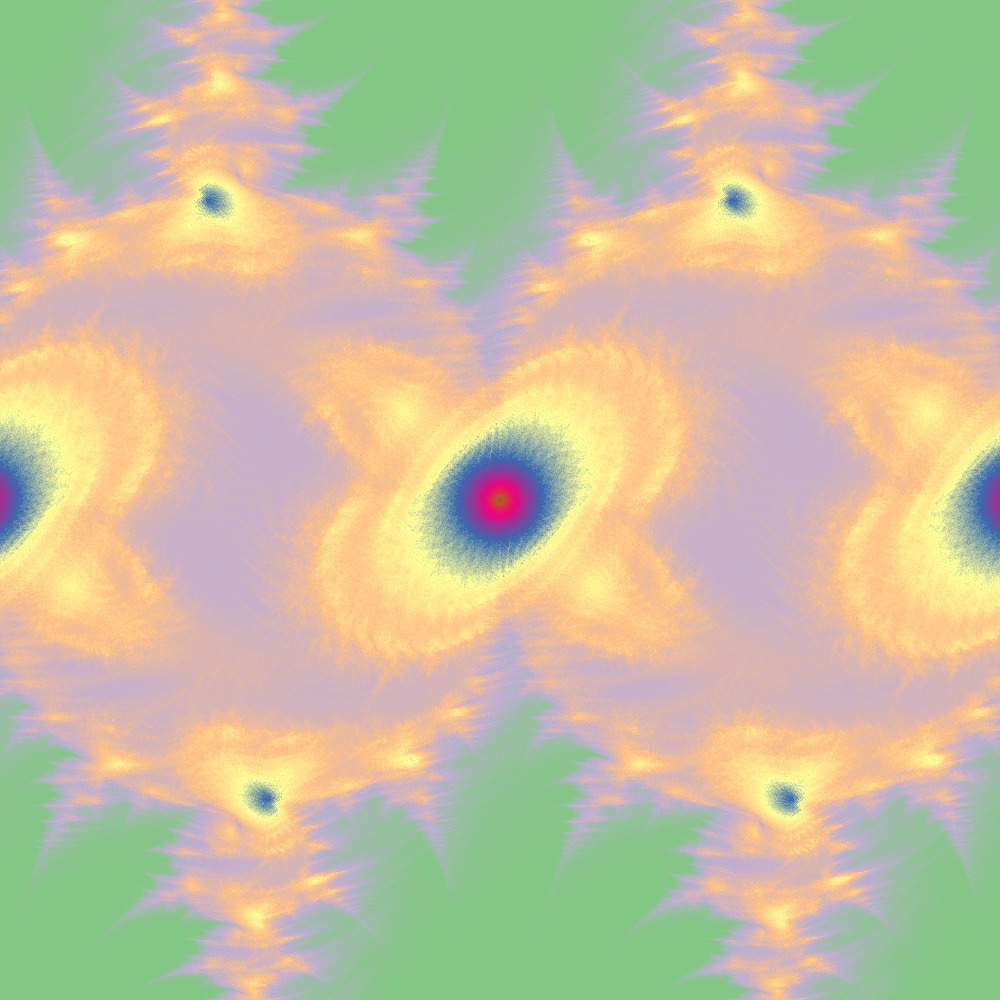
Different color scheme for Julia set for the function $c\times sin(z)$ $c=(1+[0.0..1.0]j)$ 100slices
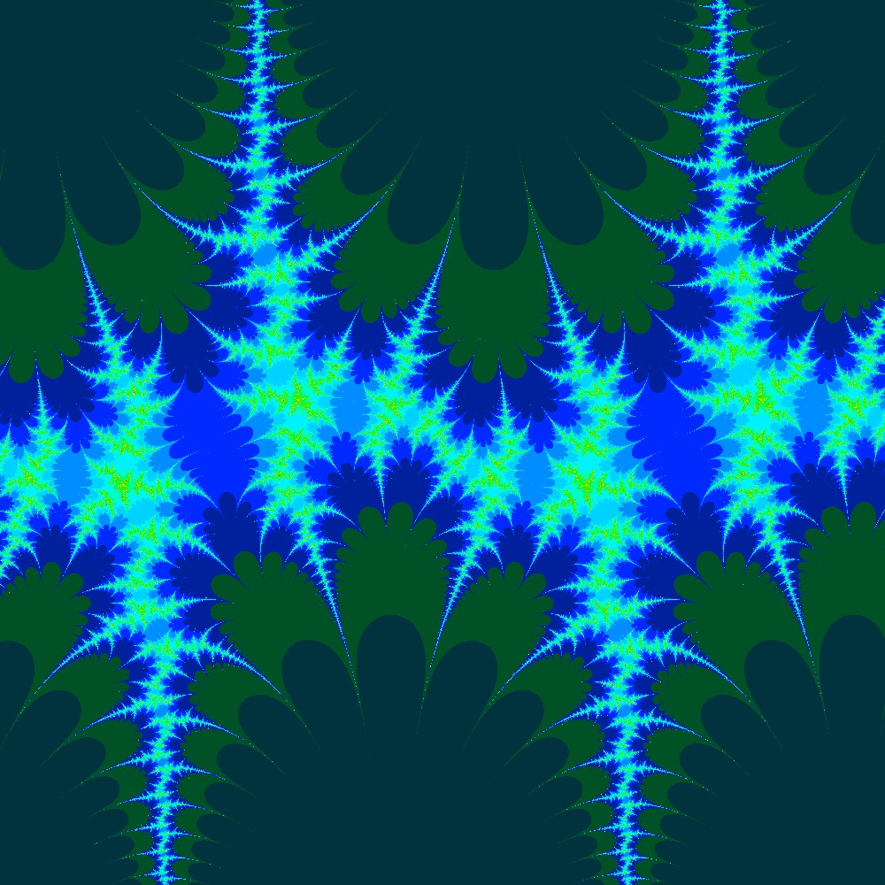
Visualization of the Julia set for the function $c\times cos(z)$ $c=\frac{\pi}{2}(1.5+0.5i)$
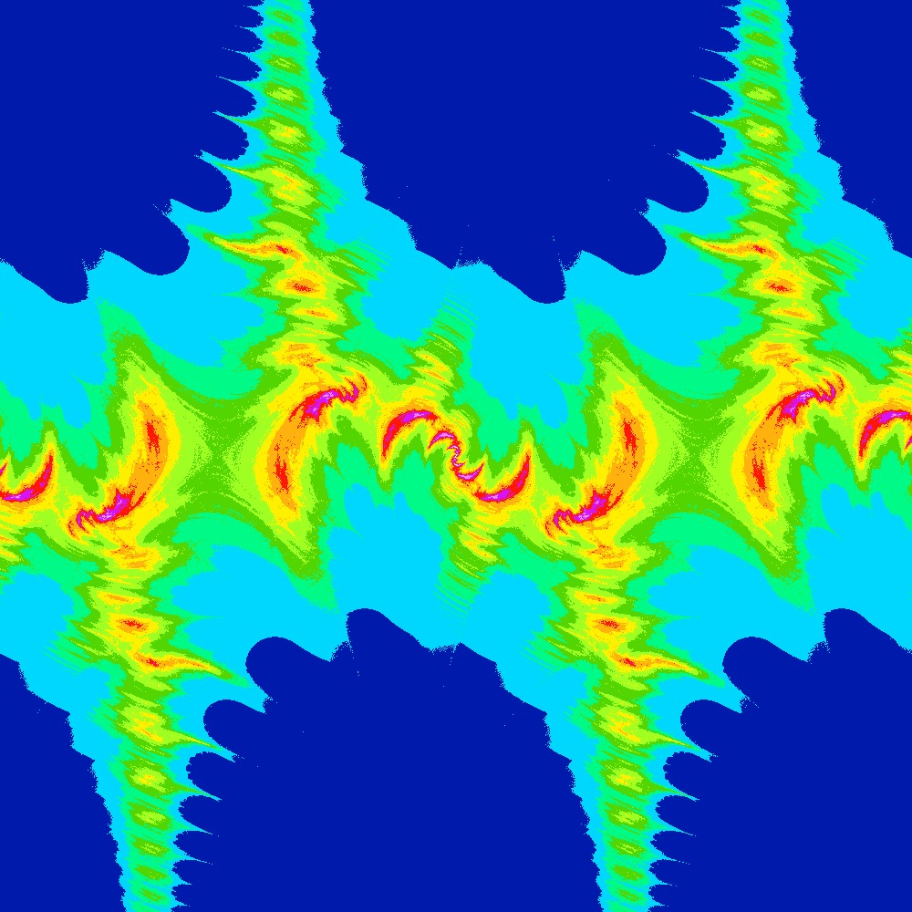
Visualization of the Julia set for the function $c\times sin(z)$ $c=\frac{\pi}{2}(1.5+0.5i)$
Visualization of the Julia set for the function $c\times sin(z)$ $c=\frac{\pi}{2}(1.5+[0.05..1.0]i)$ 100 slices
Visualization of the Julia set for the function $z^n + (−0.7 − 0.3i)$ $n=[2.0..3.0]$ 100slices
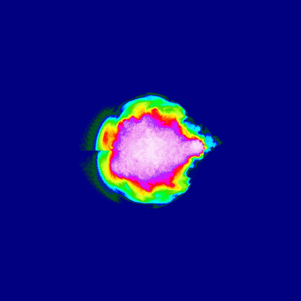
Visualization of the Julia set for the function $z^2 + (−0.7 − 0.3i)$
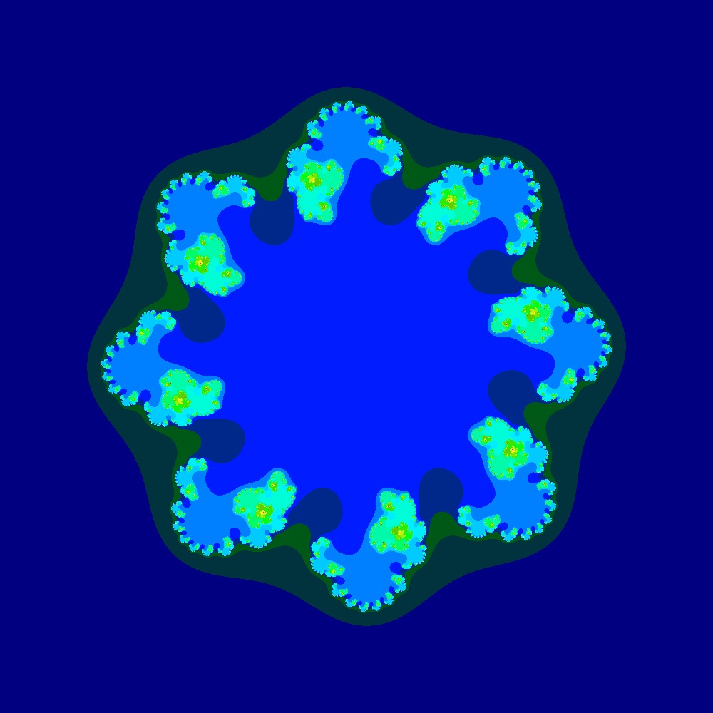
Visualization of the Julia set for the function $z^8 + (−0.7 − 0.3i)$
Visualization of the Julia set for the function $z^n + (-1 + 0i)$ $n=[2.0..3.0]$ 100slices
Future improvements
- Make the code more memory efficient so we can generate ridiculously high resolution images.
- Make the 3D modeling code more efficient.
- Find a way to visualize higher dimensions of Julia sets.
Things we learned
- Use np.zeros not np.empty if using matrix math since you may have left over junk in the memory.
- Numpy sin and cos can handle complex numbers properly.
- FDM 3D printing is finiky. It is sensitive to how well the bed is leveled and what temperature the filament is extruded at. Some filaments seem to work well at higher temperatures but eventually jam if run long enough (usually with the end in sight).
- For anything smaller then 1mm x 1mm FDM creates fragile models (large flat surfaces are generally fine).